2.1 Plots¶

How to create plots, scatter plots, and filled polygons¶

Watch this video from 4:09 to 8:12

# To load the video, execute this cell by pressing shift + enter

from IPython.display import YouTubeVideo
from datetime import timedelta
start=int(timedelta(hours=0, minutes=4, seconds=9).total_seconds())
end=int(timedelta(hours=0, minutes=8, seconds=12).total_seconds())

YouTubeVideo("PJ1dvAgOAj0",start=start,end=end,width=640,height=360)

The following is a transcript of the video.

💡 Remember: You must first import matplotlib in order to make plots. Below are the data that we will be working with in this lesson that are used in the video. These are lists of x and y coordinate values for 15 different Vitis and Ampelopsis species. Execute the cell below to read in the data to complete this lesson.

# Execute this cell to import matplotlib

import matplotlib.pyplot as plt
%matplotlib inline

# This cell contains lists of x values and y values for 
# leaf outlines of 15 Vitis and Ampelopsis species.
# Each list has the abbreviated first initial of the genus and species epithet

# Ampelopsis "acoutifolia" (actually aconitifolia)

# NOTE: There is a transcription error for this species, which is actually
# Ampelopsis aconitifolia (it is not A. "acoutifolia")
# The mistake is propagated in the videos, narration, text, and notebooks
# but it does not affect the lesson at hand for plotting in matplotlib
Aaco_x = [13.81197507,-14.58128237,-135.3576208,-3.48017966,-285.0289837,-4.874351136,-126.9904669,10.54932685,170.4482865,40.82555888,205.158889,124.6343366,13.81197507]
Aaco_y = [27.83951365,148.6870909,157.2273013,35.73510131,-30.02915903,9.54075375,-280.2095191,0.200400495,-234.1044141,20.41991159,41.33121759,96.75084391,27.83951365]

# Ampelopsis brevipedunculata
# NOTE: This species is now referred to as A. glandulosa var. brevipedunculata
Abre_x = [40.00325135,-81.37047548,-186.835592,-139.3272085,-287.5337006,-89.61277053,-134.9263008,47.43458846,144.6301719,163.5438321,225.9684307,204.719859,40.00325135]
Abre_y = [96.8926433,203.3273536,134.0172438,99.7070006,-81.35389923,-17.90701212,-335.624547,-80.02986776,-262.0385648,-27.31979918,-42.24377429,82.08218538,96.8926433]

# Ampelopsis cordata
Acor_x = [41.26484889,-99.68651819,-203.5550411,-181.4080156,-226.4063517,-174.1104713,-142.2197176,81.25359041,113.9079805,205.9930561,230.8000389,226.6914467,41.26484889]
Acor_y = [105.1580727,209.8514829,131.8410788,111.9833751,-70.79184424,-60.25829908,-326.5994491,-170.6003249,-223.0042176,-44.58524791,-45.80679706,71.64004113,105.1580727]

# Vitis acerifolia
Vace_x = [47.55748802,-102.1666218,-218.3415108,-183.5085694,-234.8755094,-152.1581487,-113.8943819,53.48770667,84.83899263,206.557697,240.589609,243.5717264,47.55748802]
Vace_y = [111.9982016,241.5287104,125.6905949,110.350904,-108.1932176,-74.67866027,-283.2678229,-161.1592736,-243.1116283,-54.52616737,-68.953011,95.74558526,111.9982016]

# Vitis aestivalis
Vaes_x = [34.13897003,-59.06591289,-192.0336456,-169.5476603,-261.8813454,-154.4511279,-132.6031657,56.04516606,119.9789735,205.0834004,246.928663,209.2801298,34.13897003]
Vaes_y = [80.26320349,227.2107718,155.0919347,123.2629647,-86.47992069,-70.12024178,-317.80585,-156.8388147,-247.9415158,-31.73423173,-28.37195726,120.2692722,80.26320349]

# Vitis amurensis
Vamu_x = [36.94310365,-63.29959989,-190.35653,-180.9243738,-255.6224889,-172.8141253,-123.8350652,60.05314983,113.598307,218.8144919,238.6851057,210.9383524,36.94310365]
Vamu_y = [87.06305005,230.9299013,148.431809,128.4087423,-88.67075769,-84.47396366,-298.5959647,-181.4317592,-241.2343437,-37.53203788,-30.63962885,115.7064075,87.06305005]

# Vitis cinerea
Vcin_x = [41.13786595,-78.14668163,-195.0747469,-185.81005,-238.1427795,-181.5728492,-127.6203541,65.24059352,103.8414516,214.1320626,233.1457326,222.7549456,41.13786595]
Vcin_y = [98.40296936,233.6652514,136.6641628,117.9719613,-86.41814245,-86.14771041,-310.2979998,-190.9232443,-230.5027809,-50.27050419,-42.94757891,107.8271097,98.40296936]

# Vitis coignetiae
Vcoi_x = [36.29348151,-51.46279315,-183.6256382,-176.7604659,-253.3454527,-191.8067468,-123.413666,66.11061054,111.4950714,215.7579824,236.7136632,197.5512918,36.29348151]
Vcoi_y = [86.42303732,222.7808161,150.0993737,127.4697835,-85.23634837,-93.3122815,-301.819185,-203.7840759,-239.8063423,-35.30522815,-25.15349577,121.1295308,86.42303732]

# Vitis labrusca
Vlab_x = [33.83997254,-63.35703212,-191.4861127,-184.3259869,-257.3706479,-179.056825,-124.0669143,68.23202857,123.213115,222.8908464,243.056641,205.2845683,33.83997254]
Vlab_y = [81.34077013,222.8158575,153.7885633,132.4995037,-80.2253417,-80.67586345,-296.8245229,-185.0516494,-238.8655248,-38.2316427,-29.21879919,111.424232,81.34077013]

# Vitis palmata
Vpal_x = [31.97986731,-68.77672824,-189.26295,-164.4563595,-260.2149738,-149.3150935,-131.5419837,65.86738801,127.3624336,202.6655429,240.0477009,219.0385121,31.97986731]
Vpal_y = [78.75737572,232.9714762,149.7873103,124.8439354,-71.09770423,-56.52814058,-329.0863141,-149.308084,-231.1263997,-33.22358667,-33.0517181,114.3110289,78.75737572]

# Vitis piasezkii
Vpia_x = [18.70342336,-28.68239983,-133.7834969,-32.76128224,-305.3467215,-7.429223951,-146.2207875,21.81934547,163.1265031,65.21695943,203.4902238,139.6214571,18.70342336]
Vpia_y = [41.05946323,160.3488167,157.9775135,64.93177072,-59.68750782,18.85909594,-362.1788431,7.556816875,-253.8796355,21.33965973,17.69878265,93.72614181,41.05946323]

# Vitis riparia
Vrip_x = [44.65674776,-85.47236587,-205.1031097,-174.088415,-239.9704675,-161.1277029,-125.4900046,58.08609552,89.2307808,204.9127104,236.0709257,229.8098573,44.65674776]
Vrip_y = [106.5948187,235.8791214,130.341464,116.8318515,-110.5506636,-76.73562488,-300.1092173,-169.0146383,-247.0956802,-42.2253331,-54.23469169,103.9732427,106.5948187]

# Vitis rupestris
Vrup_x = [51.29642881,-132.9650549,-227.6059714,-201.31783,-207.965755,-149.2265432,-98.64097334,48.33648281,75.91437502,208.7784453,237.4842778,263.3479415,51.29642881]
Vrup_y = [123.7557878,233.5830974,109.6847731,95.43848563,-95.82512925,-80.06286127,-236.7411071,-163.7331427,-213.2925544,-77.04510916,-86.40789274,69.86940263,123.7557878]

# Vitis thunbergii
Vthu_x = [22.61260382,-3.204532702,-150.3627277,-79.39836351,-271.8885204,-70.74704134,-168.6002498,36.68300146,172.978549,116.9174032,227.8346055,148.3453958,22.61260382]
Vthu_y = [50.82336098,194.3865012,181.2536906,86.8671412,-57.33457233,-23.85610668,-334.279317,-67.36542042,-234.1205595,7.151772223,28.16801823,138.9705667,50.82336098]

# Vitis vulpina
Vvul_x = [39.44771371,-83.62933643,-194.2000993,-175.9638941,-227.8323987,-180.8587446,-135.986247,71.94543538,99.8983207,207.0950158,231.7808734,222.7645396,39.44771371]
Vvul_y = [96.44934373,230.0148139,136.3702366,119.8017341,-83.09830126,-75.38247957,-332.9188424,-184.4324688,-222.8532423,-41.89574792,-44.70218529,101.9138055,96.44934373]

# Average grape leaf
avg_x = [35.60510804,-67.88314703,-186.9749654,-149.5049396,-254.2293735,-135.3520852,-130.4632741,54.4100207,120.7064692,180.696724,232.2550642,204.8782463,35.60510804]
avg_y = [84.95317026,215.7238025,143.85314,106.742536,-80.06000256,-57.00477464,-309.8290405,-137.6340316,-237.7960327,-31.10365842,-30.0828468,103.1501279,84.95317026] 

We have loaded in the data, lists of x and y values. We have imported matplotlib, so that we have the functions to create plots. So let’s actually create some plots now!

If you remember we have lists for each species. These lists are for the x values and the y values of points that make up the leaf shape for each species. Remember that when we use a function in matplotlib we have to refer to the module, abbreviated as plt for matplotlib. So we write plt dot and then we write the function plot (plt.plot()) and then we place as an argument in this function a list of values.

These are the x values for Ampelopsis aconitifolia, for its leaf, and let’s see what happens when we press shift + enter.

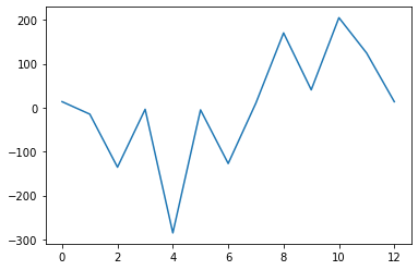
You can see that we get a plot. It should be displaying within your Jupyter notebook. The y axis is actually the x values. And the x-axis is the order of those values. The reason it looks like this is because we only have x values so it just plots values along the y-axis and their order along the x-axis just as it finds them in the list.

# just x values
# Ampelopsis acoutifolia

plt.plot(Aaco_x) 

[<matplotlib.lines.Line2D at 0x7f845a2be4f0>]

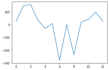
We could do this for the y values, though. So you can say plt.plot() and put in a list of y values and now you get the same thing. It’s just y values in the order that matplotlib finds them.

# just y values

plt.plot(Aaco_y) 

[<matplotlib.lines.Line2D at 0x7f8452216a90>]

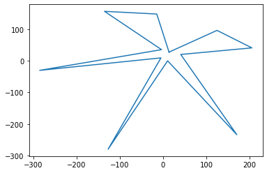
The whole point here, though, is that we’re trying to visualize leaves and we have a list of x and y values that we need to put together to have actual coordinates. This is very simple. You have your plot function and you just put a list of x values and then you put in a list of y values and now when you create the plot you can see that matplotlib puts the x and y values together and it creates a line in the order that it finds these coordinates. Here we get something that looks like a leaf. This is the tip of the leaf, this is the base of the leaf, and you can see this is a very deeply lobed leaf that looks like a star.

So this is the plot function. It creates a line connecting the points.

# Putting the x and y values together

plt.plot(Aaco_x, Aaco_y)

[<matplotlib.lines.Line2D at 0x7f8452189580>]

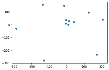
But there’s other functions. Maybe you’ve heard of something called a scatter plot. A scatter plot, if you have point data like we have here, it’ll just create points. So if we say plt.scatter() but put the same x and y values instead what we get is those points, not the line.

# Instead of plt.plot() which gives lines connecting the point
# we can use plt.scatter() instead

plt.scatter(Aaco_x, Aaco_y)

<matplotlib.collections.PathCollection at 0x7f8452167400>

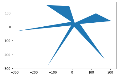
Another function is fill. So if we say plt.fill(), we won’t get lines or points back, instead we get a filled polygon.

# plt.fill() will fill in a polygon that the points make

plt.fill(Aaco_x, Aaco_y)

[<matplotlib.patches.Polygon at 0x7f84520d8280>]

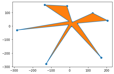
You can actually just keep on adding these functions on top of each other and you’ll see that this is one of the most powerful ways to create complex visualizations. You can use the plot function, the scatter function, and the fill function all together and you can see what you get is you get a line, an outline of the leaf connecting the points, you get the points, and you also get a filled polygon. You can just keep on adding different functions in matpotlib, executing them one after the other, and it’s just like pasting over on top of what you have already plotted.

# You can use plt.plot(), plt.scatter(), and plt.fill() together

plt.plot(Aaco_x, Aaco_y)
plt.scatter(Aaco_x, Aaco_y)
plt.fill(Aaco_x, Aaco_y)

[<matplotlib.patches.Polygon at 0x7f84520348e0>]

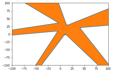
There’s numerous other functions that you can use. For example you can use plt.xlim() and plt.ylim() to modify your plot. Let’s say we wanted to limit the x and y values to just between negative and positive 100. You can see now, for example, that this cuts off our leaf.

# You can use plt.xlim() and plt.ylim() to set axes ranges

plt.plot(Aaco_x, Aaco_y)
plt.scatter(Aaco_x, Aaco_y)
plt.fill(Aaco_x, Aaco_y)
plt.xlim(-100,100)
plt.ylim(-100,100)

(-100.0, 100.0)

Plants & Python

2.1 Plots¶

How to create plots, scatter plots, and filled polygons¶