Activity 2: The shapes of leaves and sunflowers 🍃🌻
The shape of data, the shape of leaves 🍃: visualizing data using matplotlib
Lists store data, and more often than not, data is encoded numerically. Lists are a powerful tool in Python to store and manipulate data. But before analyzing data, we must know what it is, and to know our data, we need to visualize it. When we see something we first notice its form: its shape, outline, structure, and geometry. All data has a shape, and all shapes are data.
In this exercise we will learn to visualize our data using Matplotlib. Matplotlib is a module. Modules in Python are collections of functions and statements. Modules are usually designed to address a specific functionality or a niche community interest. The modules we will encounter in this course are generalist, and include matplotlib, pandas, and math.
We learned in the previous lesson that plant species are diverse and numerous, occupying the oceans, rivers, and land as single-celled organisms, large and elaborate multicellular organisms, symbionts, and even colonies. Let’s visualize some of this natural variation, using grapevine again as an example.
Wine we drink is made primarily from the berries of Vitis vinifera. But the vines themselves are chimeras: that is, most grapevines used for wine production are a surgical combination of two different species produced through grafting. The shoots may be V. vinifera, but the roots are wild relatives that are disease resistant and well-adapted for particular soil types.
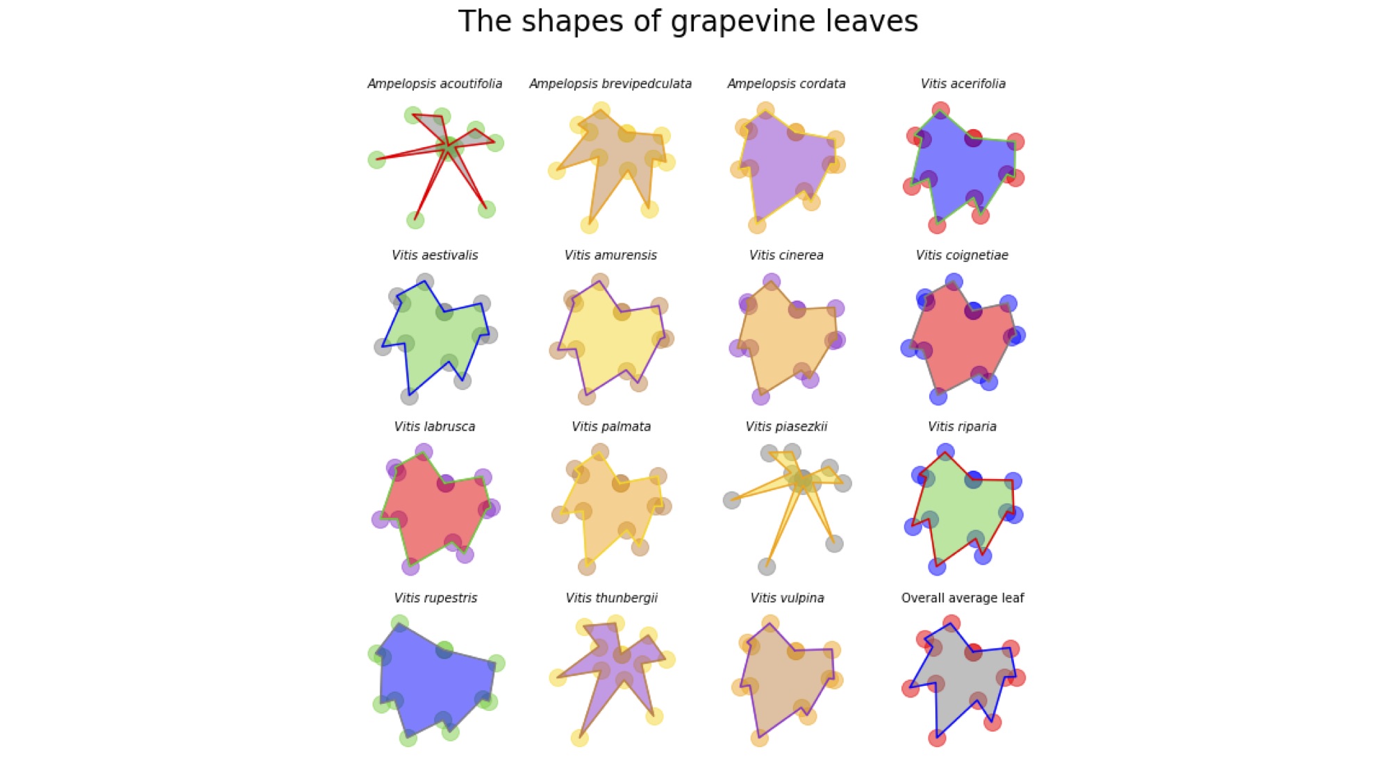
The shapes of grapevine leaves easily lend themselves to quantitative analysis. Every grapevine leaf has five major lobes: the leaf tip, two distal and two proximal lobes (proximal is near the leaf base and distal towards the tip). Additionally, there are distal and proximal sinuses (the indentations between the lobes). Some leaves are highly dissected (meaning they are very lobed) and others more entire (lacking lobing). Because these points are on every grapevine leaf, there is a correspondence between points, which allows us to compare the shapes of grapevine leaves against each other.
In the cell below are lists of x values and y values for the averaged leaves of Vitis and Ampelopsis species, as well as the overall averaged grapevine leaf. Execute the cell below to read in this data and make some graphs yourself, below!
# This cell contains lists of x values and y values for
# leaf outlines of 15 Vitis and Ampelopsis species.
# Each list has the abbreviated first initial of the genus and species epithet

# Ampelopsis acoutifolia
Aaco_x = [13.81197507,-14.58128237,-135.3576208,-3.48017966,-285.0289837,-4.874351136,-126.9904669,10.54932685,170.4482865,40.82555888,205.158889,124.6343366,13.81197507]
Aaco_y = [27.83951365,148.6870909,157.2273013,35.73510131,-30.02915903,9.54075375,-280.2095191,0.200400495,-234.1044141,20.41991159,41.33121759,96.75084391,27.83951365]

# Ampelopsis brevipedunculata
Abre_x = [40.00325135,-81.37047548,-186.835592,-139.3272085,-287.5337006,-89.61277053,-134.9263008,47.43458846,144.6301719,163.5438321,225.9684307,204.719859,40.00325135]
Abre_y = [96.8926433,203.3273536,134.0172438,99.7070006,-81.35389923,-17.90701212,-335.624547,-80.02986776,-262.0385648,-27.31979918,-42.24377429,82.08218538,96.8926433]

# Ampelopsis cordata
Acor_x = [41.26484889,-99.68651819,-203.5550411,-181.4080156,-226.4063517,-174.1104713,-142.2197176,81.25359041,113.9079805,205.9930561,230.8000389,226.6914467,41.26484889]
Acor_y = [105.1580727,209.8514829,131.8410788,111.9833751,-70.79184424,-60.25829908,-326.5994491,-170.6003249,-223.0042176,-44.58524791,-45.80679706,71.64004113,105.1580727]

# Vitis acerifolia
Vace_x = [47.55748802,-102.1666218,-218.3415108,-183.5085694,-234.8755094,-152.1581487,-113.8943819,53.48770667,84.83899263,206.557697,240.589609,243.5717264,47.55748802]
Vace_y = [111.9982016,241.5287104,125.6905949,110.350904,-108.1932176,-74.67866027,-283.2678229,-161.1592736,-243.1116283,-54.52616737,-68.953011,95.74558526,111.9982016]

# Vitis aestivalis
Vaes_x = [34.13897003,-59.06591289,-192.0336456,-169.5476603,-261.8813454,-154.4511279,-132.6031657,56.04516606,119.9789735,205.0834004,246.928663,209.2801298,34.13897003]
Vaes_y = [80.26320349,227.2107718,155.0919347,123.2629647,-86.47992069,-70.12024178,-317.80585,-156.8388147,-247.9415158,-31.73423173,-28.37195726,120.2692722,80.26320349]

# Vitis amurensis
Vamu_x = [36.94310365,-63.29959989,-190.35653,-180.9243738,-255.6224889,-172.8141253,-123.8350652,60.05314983,113.598307,218.8144919,238.6851057,210.9383524,36.94310365]
Vamu_y = [87.06305005,230.9299013,148.431809,128.4087423,-88.67075769,-84.47396366,-298.5959647,-181.4317592,-241.2343437,-37.53203788,-30.63962885,115.7064075,87.06305005]

# Vitis cinerea
Vcin_x = [41.13786595,-78.14668163,-195.0747469,-185.81005,-238.1427795,-181.5728492,-127.6203541,65.24059352,103.8414516,214.1320626,233.1457326,222.7549456,41.13786595]
Vcin_y = [98.40296936,233.6652514,136.6641628,117.9719613,-86.41814245,-86.14771041,-310.2979998,-190.9232443,-230.5027809,-50.27050419,-42.94757891,107.8271097,98.40296936]

# Vitis coignetiae
Vcoi_x = [36.29348151,-51.46279315,-183.6256382,-176.7604659,-253.3454527,-191.8067468,-123.413666,66.11061054,111.4950714,215.7579824,236.7136632,197.5512918,36.29348151]
Vcoi_y = [86.42303732,222.7808161,150.0993737,127.4697835,-85.23634837,-93.3122815,-301.819185,-203.7840759,-239.8063423,-35.30522815,-25.15349577,121.1295308,86.42303732]

# Vitis labrusca
Vlab_x = [33.83997254,-63.35703212,-191.4861127,-184.3259869,-257.3706479,-179.056825,-124.0669143,68.23202857,123.213115,222.8908464,243.056641,205.2845683,33.83997254]
Vlab_y = [81.34077013,222.8158575,153.7885633,132.4995037,-80.2253417,-80.67586345,-296.8245229,-185.0516494,-238.8655248,-38.2316427,-29.21879919,111.424232,81.34077013]

# Vitis palmata
Vpal_x = [31.97986731,-68.77672824,-189.26295,-164.4563595,-260.2149738,-149.3150935,-131.5419837,65.86738801,127.3624336,202.6655429,240.0477009,219.0385121,31.97986731]
Vpal_y = [78.75737572,232.9714762,149.7873103,124.8439354,-71.09770423,-56.52814058,-329.0863141,-149.308084,-231.1263997,-33.22358667,-33.0517181,114.3110289,78.75737572]

# Vitis piasezkii
Vpia_x = [18.70342336,-28.68239983,-133.7834969,-32.76128224,-305.3467215,-7.429223951,-146.2207875,21.81934547,163.1265031,65.21695943,203.4902238,139.6214571,18.70342336]
Vpia_y = [41.05946323,160.3488167,157.9775135,64.93177072,-59.68750782,18.85909594,-362.1788431,7.556816875,-253.8796355,21.33965973,17.69878265,93.72614181,41.05946323]

# Vitis riparia
Vrip_x = [44.65674776,-85.47236587,-205.1031097,-174.088415,-239.9704675,-161.1277029,-125.4900046,58.08609552,89.2307808,204.9127104,236.0709257,229.8098573,44.65674776]
Vrip_y = [106.5948187,235.8791214,130.341464,116.8318515,-110.5506636,-76.73562488,-300.1092173,-169.0146383,-247.0956802,-42.2253331,-54.23469169,103.9732427,106.5948187]

# Vitis rupestris
Vrup_x = [51.29642881,-132.9650549,-227.6059714,-201.31783,-207.965755,-149.2265432,-98.64097334,48.33648281,75.91437502,208.7784453,237.4842778,263.3479415,51.29642881]
Vrup_y = [123.7557878,233.5830974,109.6847731,95.43848563,-95.82512925,-80.06286127,-236.7411071,-163.7331427,-213.2925544,-77.04510916,-86.40789274,69.86940263,123.7557878]

# Vitis thunbergii
Vthu_x = [22.61260382,-3.204532702,-150.3627277,-79.39836351,-271.8885204,-70.74704134,-168.6002498,36.68300146,172.978549,116.9174032,227.8346055,148.3453958,22.61260382]
Vthu_y = [50.82336098,194.3865012,181.2536906,86.8671412,-57.33457233,-23.85610668,-334.279317,-67.36542042,-234.1205595,7.151772223,28.16801823,138.9705667,50.82336098]

# Vitis vulpina
Vvul_x = [39.44771371,-83.62933643,-194.2000993,-175.9638941,-227.8323987,-180.8587446,-135.986247,71.94543538,99.8983207,207.0950158,231.7808734,222.7645396,39.44771371]
Vvul_y = [96.44934373,230.0148139,136.3702366,119.8017341,-83.09830126,-75.38247957,-332.9188424,-184.4324688,-222.8532423,-41.89574792,-44.70218529,101.9138055,96.44934373]

# Average grape leaf
avg_x = [35.60510804,-67.88314703,-186.9749654,-149.5049396,-254.2293735,-135.3520852,-130.4632741,54.4100207,120.7064692,180.696724,232.2550642,204.8782463,35.60510804]
avg_y = [84.95317026,215.7238025,143.85314,106.742536,-80.06000256,-57.00477464,-309.8290405,-137.6340316,-237.7960327,-31.10365842,-30.0828468,103.1501279,84.95317026]
In the previous lesson, you plotted the leaf from one species. In this activity, let’s plot them all!
Using subplots, plot each of the 15 species plus the overall average grapevine leaf. Your plot will have 4 rows and 4 columns. Give your overall figure a title. For each subplot, use the species name as the title and make it italic (don’t use italics for the overall averaged leaf and give it an appropriate title as well). Turn off the axes for your figure. Plot the outline, points, and fill for each leaf. Use alpha appropriately to better visualize the shapes.
First, always import matplotlib!
Remember, the general structure of the code to call a subplot is:
fig = plt.figure(figsize=(width, height))

ax_array = fig.subplots(nrows, ncols)
You then refer to a specific subplot by indexing the rows and columns using the array you created (for example, ax_array[row, col].
Also, after coding your figure, be sure to save your figure using the code below! You just add a single line after the code for your graph. You can use a variety of file formats, but give the file name as either .jpg, .pdf, .png, or .tiff (.jpgis only given here as an example). The file will be saved in your home directory (or wherever you are running Jupyter from) in the format that you specify. You can provide a path to a different directory you wish to save to as well (for example, ./Desktop/my_file.jpg).
plt.savefig("the_file_name.jpg")
Be creative and have fun with this figure! It is meant for you to explore the functionality of matplotlib. There are no wrong answers!
Hint: to save yourself some time, first specify the overall 4 x 4 subplot, but only code the first graph. See how the sizes of your different parameters work. Then, copy and paste that code and just replace with different parameters. This will save you time rather than writing everything out or going back and changing the font size for each subplot! Alternatively, create a variable at the beginning of your code for a parameter (like scatterplot point size) and set this attribute to the parameter value. Then, if you need to change the value, you can change for all subplots at once.
# Put your answer here
Below, an example of a possible graph you might make. Again, be creative in your use of matplotlib!
The shape of sunflowers 🌻
In the next lesson and activity, we will be learning about loops, a way to automate repetitive tasks. We will be using loops to calculate the Fibonacci sequence, the Golden angle, and to model sunflower growth. In many ways, plants are the computers, iteratively producing leaves and other organs in a precise mathematical order. When we use Python to model their growth, we are the ones following their lead.
The ability to visualize and look at data is foundational to all of your computational work. In this exercise, you will visualize the points on a sunflower as a preview to the next lessons using the different funcitons of matplotlib. You will also use the indexing and slicing techniques you learned in the previous lesson to look at “parastichies”, or the curves that emerge when looking at a sunflower pattern.
You will be using loops to generate the data below in the next lesson! But for now execute the cell below to load in the x and y coordinates of a sunflower.
sun_xlist = [0.0,-0.7373688780783197,0.12363864559502138,1.053847020514727,-1.9694269706308574,1.8866941955758958,
 -0.6358980820385529,-1.2194453649142762,2.6568018333748893,-2.7730366684134142,1.3403187214918457,
 0.9926122841712306,-2.997179549141454,3.5214545813198486,-2.1519372768917857,-0.4977197614011282,
 3.0585959818241726,-4.119584716091113,3.0073085133506017,-0.20134384491006577,-2.8653384038891687,
 4.541650602805144,-3.8501668802872424,1.0525956694116372,2.4356789070709124,-4.7634638859834535,
 4.628844704413331,-2.006032227609403,-1.7909211243064767,4.766891005951,-5.296312842870197,
 3.0112570857032295,0.9581363211912816,-4.541784358263451,5.811043126965286,-4.017487592669849,
 0.029269662980670484,4.0869179180944695,-6.13810860306323,4.974512119299716,-1.131991572873186,
 -3.4103397878411568,6.250267164954252,-5.834063230160405,2.305829117107365,2.5292790181008407,
 -6.128892214086734,6.5513509901593245,-3.503054434163048,-1.4696666530084994,5.764667212478689,
 -7.086605355446326,4.674016622598716,0.2653106694985794,-5.157991090299893,7.406523200751739,
 -5.76888817488349,1.043236970610896,4.319062423897526,-7.48554069915315,6.739471132676982,
 -2.4100779669432555,-3.267627295640393,7.306868734670486,-7.5409873950070185,3.785580104670517,
 2.0323907649727597,-6.86324298562459,8.13378251542539,-5.1181480476641,-0.6501056102210901,
 6.157353364008793,-8.484877515776738,6.356090828162586,-0.8356354241304721,-5.201930418721218,
 8.569309573315453,-7.449520848340097,2.3758663326403617,4.019479292270886,-8.371210207962406,
 8.352217739526045,-3.917926138387042,-2.6416647522428898,7.884578820243296,-9.0233911389071,
 5.4072932931621756,1.1083634450004225,-7.113719950202413,9.42927937071088,-6.789514554197385,
 0.5335884843254842,6.073324177924158,-9.544526094990951,8.012162670581947,-2.2319132418077428,
 -4.788184831492389,9.35328406571534,-9.026755434325707,3.9306258386646395]

sun_ylist = [0.0,0.6754902942615238,-1.4087985964343621,1.3745568221620497,-0.3483639007586233,-1.2001604111035422,
 2.3655091691345627,-2.347967845177844,0.9702597684001061,1.1446692254248088,-2.864183256151475,
 3.1646043754808235,-1.7369268119895633,-0.7741819112466066,3.0609093348747796,-3.8408690473785754,
 2.577787931535297,0.17035776163269098,-2.992673638325601,4.354246278762472,-3.4336330367699275,
 0.6110726651059321,2.6788458324321702,-4.678893283324152,4.250584461182937,-1.519674901724516,
 -2.1386436595245724,4.79331145470357,-4.97921695917268,2.5053443151358374,1.3960910681070222,
 -4.683196639454945,5.575121056086051,-3.5174130896204754,-0.48143304472118015,4.342786368536199,
 -5.999928606811,4.505230508060421,-0.5688785256987186,-3.7754773439844995,6.222426783735112,
 -5.419371045745764,1.7129391018640276,2.993944927097081,-6.2195781273893385,6.213110947713299,
 -2.904596396766168,-2.0198515301225584,5.977341351411227,-6.843981292276798,4.09494956371543,
 0.8831899773884733,-5.49122651250801,7.275273895094961,-5.23403552838409,0.37870051059672993,
 4.766542691059153,-7.47740975359453,6.272615066977762,-1.7224054230412074,-3.818314923079766,
 7.429099823885439,-7.163980168648281,3.0999466599112546,2.67086298943717,-7.118242990452261,
 7.865709616967401,-4.46048155699302,-1.3570490012376957,6.5425194353698455,-8.341304615919446,
 5.752130001202128,-0.08278612363409138,-5.709650548338964,8.561641982583614,-6.923865966263566,
 1.6021652338894832,4.637309471034498,-8.506189462351873,7.927407282271141,-3.1500539128887963,
 -3.352679351137899,8.163936230406483,-8.719037064765669,4.6726241906845924,1.8916691979024318,
 -7.5340015424556,9.261292052072799,-6.115144190457997,-0.2978095852826337,6.625895571041086,
 -9.52445711468088,7.423929783466559,-1.3791379996348347,-5.4594184067657965,9.48781130087668,
 -8.548291409367499,3.0848139629539255,4.064195655830474,-9.140578784542141]
In the cell below, use the plt.plot() function using the \(x\) and \(y\) values from the lists sun_xlist and sun_ylist to plot the respective \(x\) and \(y\) coordinates. Adjust the linewidth, linestyle, color, and alpha to your liking and to highlight any patterns that you see. Remember to set an equal aspect ratio as well using plt.axes().set_aspect('equal', 'box')).
What patterns do you see? Do you see different patterns using different linewidths?
# Put your answer here
Maybe lines are not the best way to visualize sunflowers. Use plt.scatter() to visualize the same data, again choosing a color, point size, and alpha that reveals the patterns that you see.
# Put your answer here
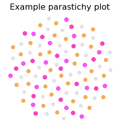
If you remember, every nth term of the Fibonacci sequence is divisible by the nth term. When you look at a sunflower, part of the pattern you see are “arms” or “arcs” radiating as curves from the center of the sunflower to the edges. The arcs are called parastichies. They are defined by taking every nth point in the sunflower, where \(n\) is a Fibonacci sequence number. If you plot every nth term of the next number in the Fibonacci sequence, it will yield arms that curve in opposite direction.
In the cell below, use plt.scatter() again to plot out all the points of the sunflower. But in the next lines, use slicing to select every nth element where \(n\) is a term of the Fibonacci sequence. After using plt.scatter() to plot every nth term, use plt.scatter() again on the line after that to plot every nth term of the next term in the Fibonacci sequence. Use alpha and colors to make the plot of all points less conspicuous, and use alpha = 1 and increases in point size for the parastichy plots to highlight them. Use different colors for the opposite handed parastiches.
For slicing, you should begin with the 1st term of the sunflower points, include all points to the end, and choose two successive terms of the Fibonacci sequence for your steps.
Remember, for each parastichy, you must use the same slicing (there must be the same number of \(x\) and \(y\) values for matplotlib to plot the points).
Your answer should resemble the plot below. Put the code for your parastichies in the following cell after.
# Put your answer here