2.4 Subplots
How to create subplots
Watch this video from 19:11 to 26:34
# To load the video, execute this cell by pressing shift + enter

from IPython.display import YouTubeVideo
from datetime import timedelta
start=int(timedelta(hours=0, minutes=19, seconds=11).total_seconds())
end=int(timedelta(hours=0, minutes=19, seconds=11).total_seconds())

YouTubeVideo("PJ1dvAgOAj0",start=start,end=end,width=640,height=360)
The following is a transcript of the video.
💡 Remember: You must first import
matplotlibin order to make plots. Below are the data that we will be working with in this lesson that are used in the video. These are lists ofxandycoordinate values for 15 different Vitis and Ampelopsis species. Execute the cell below to read in the data to complete this lesson.
# Execute this cell to import matplotlib

import matplotlib.pyplot as plt
%matplotlib inline
# This cell contains lists of x values and y values for
# leaf outlines of 15 Vitis and Ampelopsis species.
# Each list has the abbreviated first initial of the genus and species epithet

# Ampelopsis "acoutifolia" (actually aconitifolia)

# NOTE: There is a transcription error for this species, which is actually
# Ampelopsis aconitifolia (it is not A. "acoutifolia")
# The mistake is propagated in the videos, narration, text, and notebooks
# but it does not affect the lesson at hand for plotting in matplotlib
Aaco_x = [13.81197507,-14.58128237,-135.3576208,-3.48017966,-285.0289837,-4.874351136,-126.9904669,10.54932685,170.4482865,40.82555888,205.158889,124.6343366,13.81197507]
Aaco_y = [27.83951365,148.6870909,157.2273013,35.73510131,-30.02915903,9.54075375,-280.2095191,0.200400495,-234.1044141,20.41991159,41.33121759,96.75084391,27.83951365]

# Ampelopsis brevipedunculata
# NOTE: This species is now referred to as A. glandulosa var. brevipedunculata
Abre_x = [40.00325135,-81.37047548,-186.835592,-139.3272085,-287.5337006,-89.61277053,-134.9263008,47.43458846,144.6301719,163.5438321,225.9684307,204.719859,40.00325135]
Abre_y = [96.8926433,203.3273536,134.0172438,99.7070006,-81.35389923,-17.90701212,-335.624547,-80.02986776,-262.0385648,-27.31979918,-42.24377429,82.08218538,96.8926433]

# Ampelopsis cordata
Acor_x = [41.26484889,-99.68651819,-203.5550411,-181.4080156,-226.4063517,-174.1104713,-142.2197176,81.25359041,113.9079805,205.9930561,230.8000389,226.6914467,41.26484889]
Acor_y = [105.1580727,209.8514829,131.8410788,111.9833751,-70.79184424,-60.25829908,-326.5994491,-170.6003249,-223.0042176,-44.58524791,-45.80679706,71.64004113,105.1580727]

# Vitis acerifolia
Vace_x = [47.55748802,-102.1666218,-218.3415108,-183.5085694,-234.8755094,-152.1581487,-113.8943819,53.48770667,84.83899263,206.557697,240.589609,243.5717264,47.55748802]
Vace_y = [111.9982016,241.5287104,125.6905949,110.350904,-108.1932176,-74.67866027,-283.2678229,-161.1592736,-243.1116283,-54.52616737,-68.953011,95.74558526,111.9982016]

# Vitis aestivalis
Vaes_x = [34.13897003,-59.06591289,-192.0336456,-169.5476603,-261.8813454,-154.4511279,-132.6031657,56.04516606,119.9789735,205.0834004,246.928663,209.2801298,34.13897003]
Vaes_y = [80.26320349,227.2107718,155.0919347,123.2629647,-86.47992069,-70.12024178,-317.80585,-156.8388147,-247.9415158,-31.73423173,-28.37195726,120.2692722,80.26320349]

# Vitis amurensis
Vamu_x = [36.94310365,-63.29959989,-190.35653,-180.9243738,-255.6224889,-172.8141253,-123.8350652,60.05314983,113.598307,218.8144919,238.6851057,210.9383524,36.94310365]
Vamu_y = [87.06305005,230.9299013,148.431809,128.4087423,-88.67075769,-84.47396366,-298.5959647,-181.4317592,-241.2343437,-37.53203788,-30.63962885,115.7064075,87.06305005]

# Vitis cinerea
Vcin_x = [41.13786595,-78.14668163,-195.0747469,-185.81005,-238.1427795,-181.5728492,-127.6203541,65.24059352,103.8414516,214.1320626,233.1457326,222.7549456,41.13786595]
Vcin_y = [98.40296936,233.6652514,136.6641628,117.9719613,-86.41814245,-86.14771041,-310.2979998,-190.9232443,-230.5027809,-50.27050419,-42.94757891,107.8271097,98.40296936]

# Vitis coignetiae
Vcoi_x = [36.29348151,-51.46279315,-183.6256382,-176.7604659,-253.3454527,-191.8067468,-123.413666,66.11061054,111.4950714,215.7579824,236.7136632,197.5512918,36.29348151]
Vcoi_y = [86.42303732,222.7808161,150.0993737,127.4697835,-85.23634837,-93.3122815,-301.819185,-203.7840759,-239.8063423,-35.30522815,-25.15349577,121.1295308,86.42303732]

# Vitis labrusca
Vlab_x = [33.83997254,-63.35703212,-191.4861127,-184.3259869,-257.3706479,-179.056825,-124.0669143,68.23202857,123.213115,222.8908464,243.056641,205.2845683,33.83997254]
Vlab_y = [81.34077013,222.8158575,153.7885633,132.4995037,-80.2253417,-80.67586345,-296.8245229,-185.0516494,-238.8655248,-38.2316427,-29.21879919,111.424232,81.34077013]

# Vitis palmata
Vpal_x = [31.97986731,-68.77672824,-189.26295,-164.4563595,-260.2149738,-149.3150935,-131.5419837,65.86738801,127.3624336,202.6655429,240.0477009,219.0385121,31.97986731]
Vpal_y = [78.75737572,232.9714762,149.7873103,124.8439354,-71.09770423,-56.52814058,-329.0863141,-149.308084,-231.1263997,-33.22358667,-33.0517181,114.3110289,78.75737572]

# Vitis piasezkii
Vpia_x = [18.70342336,-28.68239983,-133.7834969,-32.76128224,-305.3467215,-7.429223951,-146.2207875,21.81934547,163.1265031,65.21695943,203.4902238,139.6214571,18.70342336]
Vpia_y = [41.05946323,160.3488167,157.9775135,64.93177072,-59.68750782,18.85909594,-362.1788431,7.556816875,-253.8796355,21.33965973,17.69878265,93.72614181,41.05946323]

# Vitis riparia
Vrip_x = [44.65674776,-85.47236587,-205.1031097,-174.088415,-239.9704675,-161.1277029,-125.4900046,58.08609552,89.2307808,204.9127104,236.0709257,229.8098573,44.65674776]
Vrip_y = [106.5948187,235.8791214,130.341464,116.8318515,-110.5506636,-76.73562488,-300.1092173,-169.0146383,-247.0956802,-42.2253331,-54.23469169,103.9732427,106.5948187]

# Vitis rupestris
Vrup_x = [51.29642881,-132.9650549,-227.6059714,-201.31783,-207.965755,-149.2265432,-98.64097334,48.33648281,75.91437502,208.7784453,237.4842778,263.3479415,51.29642881]
Vrup_y = [123.7557878,233.5830974,109.6847731,95.43848563,-95.82512925,-80.06286127,-236.7411071,-163.7331427,-213.2925544,-77.04510916,-86.40789274,69.86940263,123.7557878]

# Vitis thunbergii
Vthu_x = [22.61260382,-3.204532702,-150.3627277,-79.39836351,-271.8885204,-70.74704134,-168.6002498,36.68300146,172.978549,116.9174032,227.8346055,148.3453958,22.61260382]
Vthu_y = [50.82336098,194.3865012,181.2536906,86.8671412,-57.33457233,-23.85610668,-334.279317,-67.36542042,-234.1205595,7.151772223,28.16801823,138.9705667,50.82336098]

# Vitis vulpina
Vvul_x = [39.44771371,-83.62933643,-194.2000993,-175.9638941,-227.8323987,-180.8587446,-135.986247,71.94543538,99.8983207,207.0950158,231.7808734,222.7645396,39.44771371]
Vvul_y = [96.44934373,230.0148139,136.3702366,119.8017341,-83.09830126,-75.38247957,-332.9188424,-184.4324688,-222.8532423,-41.89574792,-44.70218529,101.9138055,96.44934373]

# Average grape leaf
avg_x = [35.60510804,-67.88314703,-186.9749654,-149.5049396,-254.2293735,-135.3520852,-130.4632741,54.4100207,120.7064692,180.696724,232.2550642,204.8782463,35.60510804]
avg_y = [84.95317026,215.7238025,143.85314,106.742536,-80.06000256,-57.00477464,-309.8290405,-137.6340316,-237.7960327,-31.10365842,-30.0828468,103.1501279,84.95317026]
And finally let’s talk about subplots. What if we wanted to create one plot but it had multiple panels, multiple plots within that plot, and this is where subplots comes into play.
I will not lie, the code for subplots is a little complicated. I myself often just go and look it up each time that I want to use it and you should do the same. I will put it in the notebooks whenever you need to use it in the class but this is the general outline of what a subplot looks like. Let’s go over it so we know how to use it when we need it.
An alternative way to create a plot in matplotlib is to actually create a variable that is your figure. You can use a function called plt.figure() and assign it to a variable. Usually we call it fig where you store all the elements of your figure. You can put other attributes into this. For example figsize. This is saying to create a 10 inch by 10 inch figure, using this argument when we create the figure itself.
Once you have your figure, then you use the dot subplots function to create what we call an array. What we’re doing here is we’re modifying the figure that we just created using this function subplots. The most important thing to know about the subplots is that you need to specify how many subplots you want. In this case let’s create a two by two subplot. Always rows are first followed by columns. So this is a 2x2 subplot. Remember: rows followed by columns. This is creating another variable and it’s called an array. You learned about indexing before, how if you have a list for example there’s a start and end and every element in that list has a number and index associated with it. An array is a two-dimensional indexing scheme. Remember we were specifying two rows and two columns and that’s basically what this variable is, an array.
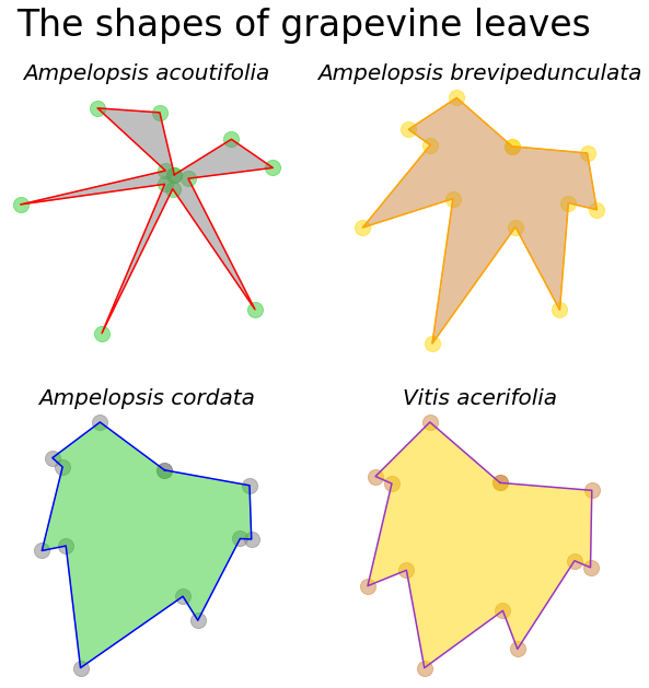
Once we have these two lines of code we have created our subplots and we can get to business creating our subplot. You can modify the figure directly. This is called “superior title”, the title on the top for the overall figure, because it’s modifying the figure directly. We’re going to call our overall figure title “The shape of grapevine leaves”. We can give it a font size and modify it like we want.
But to create the subplots, this is where all the magic happens. Previously, you created this array and remember this is two dimensional indexing. The first value separated by the comma in the square brackets is the rows. Because we have only two rows, it’s either the top or the bottom row, 0 or 1. The second value is going to refer to the columns going from left to right. It’s either the first column, 0, or it’s the second one, 1. So we can refer any of the subplots: we have four of them. The one in the upper left corner is 0, 0; the one in the upper right corner is 0, 1; the one in the lower left corner as 1, 0; and the one in the lower right corner as 1, 1. When you index two dimensionally, indexing the array object like this, by 0, 0 for example, the functions that you use, .plot(), .fill(), .scatter(), these will all modify just this one subplot. You can set a title even for just this one subplot. You can modify its aspect ratio, turn the axis off, and on, etc.
For example, this is the plot that we will create in the upper left hand corner of our subplot. And you just go about creating the plot that you would like for the upper right hand corner, the lower left hand corner, and the lower right hand corner. You can see that this is a lot of code and we did a lot of things here. We created a figure object, then we modified the figure object with subplots to create an array. This array allows us through two-dimensional indexing to refer to each of the plots that we want to create.
This is a lot but you can always look up the skeleton of how to make a subplots online and just copy and paste it from when you’ve used it before or even from this notebook. So let’s execute the cell and this is what our subplot looks like. We created the overall figure, we can create a title for the overall figure, “The shapes of grapevine leaves”. But because we created this array with two rows and two columns, when we refer to an index in that array object, we can modify each of these plots as we would like independently of each other. This creates a single, overall plot with subplots and this is how we can control and create different plots within an overall plot.
# Create an variable "fig" using plt.figure()
# Note you can use figsize to adjust size
fig = plt.figure(figsize=(10,10))

# Then, use the .subplots() function on your new fig
# Specify how many rows and how many columns separated by a comma
# This is indexing in 2 dimensions: an array
# This creates an array that holds each of your subplots
# Each plot is indexed by row, column
ax_array = fig.subplots(2,2)

# You can give your overall figure a title
# by modifying fig with .suptitle()
fig.suptitle("The shapes of grapevine leaves", fontsize=33)

# Then using indexing, refer to each subplot in your array
# Specify the way you want each plot independently
ax_array[0,0].plot(Aaco_x, Aaco_y, color="red")
ax_array[0,0].fill(Aaco_x, Aaco_y, color="gray", alpha=0.5)
ax_array[0,0].scatter(Aaco_x, Aaco_y, color="limegreen", s=200, alpha=0.5)
ax_array[0,0].set_title("Ampelopsis acoutifolia", fontsize=20, style="italic")
ax_array[0,0].set_aspect("equal", "datalim")
ax_array[0,0].axis("off")

ax_array[0,1].plot(Abre_x, Abre_y, color="orange")
ax_array[0,1].fill(Abre_x, Abre_y, color="peru", alpha=0.5)
ax_array[0,1].scatter(Abre_x, Abre_y, color="gold", s=200, alpha=0.5)
ax_array[0,1].set_title("Ampelopsis brevipedunculata", fontsize=20, style="italic")
ax_array[0,1].set_aspect("equal", "datalim")
ax_array[0,1].axis("off")

ax_array[1,0].plot(Acor_x, Acor_y, color="blue")
ax_array[1,0].fill(Acor_x, Acor_y, color="limegreen", alpha=0.5)
ax_array[1,0].scatter(Acor_x, Acor_y, color="gray", s=200, alpha=0.5)
ax_array[1,0].set_title("Ampelopsis cordata", fontsize=20, style="italic")
ax_array[1,0].set_aspect("equal", "datalim")
ax_array[1,0].axis("off")

ax_array[1,1].plot(Vace_x, Vace_y, color="darkorchid")
ax_array[1,1].fill(Vace_x, Vace_y, color="gold", alpha=0.5)
ax_array[1,1].scatter(Vace_x, Vace_y, color="peru", s=200, alpha=0.5)
ax_array[1,1].set_title("Vitis acerifolia", fontsize=20, style="italic")
ax_array[1,1].set_aspect("equal", "datalim")
ax_array[1,1].axis("off")
(-258.79787119, 267.49408819, -309.507649565, 267.768537065)
So what did we learn?
Python learning objectives
Lists can store numerical data that can be plotted
How to load in modules, sets of functionalities that allow us to do tasks in Python
How to create plots, scatter plots, filled polygons
How to manipulate shape, size, and color in plots
How to plot data on top of each other and use a legend
How to create subplots
Plant learning objectives
Phenotype is what a plant is
Phenotype can be measured
Genetic differences between closely related species results in variation
Morphology is one aspect of phenotype that can be measured using geometry