2.3 Legends
How to plot data on top of each other and use a legend
Watch this video from 16:55 to 19:11
# To load the video, execute this cell by pressing shift + enter

from IPython.display import YouTubeVideo
from datetime import timedelta
start=int(timedelta(hours=0, minutes=16, seconds=55).total_seconds())
end=int(timedelta(hours=0, minutes=19, seconds=11).total_seconds())

YouTubeVideo("PJ1dvAgOAj0",start=start,end=end,width=640,height=360)
The following is a transcript of the video.
💡 Remember: You must first import
matplotlibin order to make plots. Below are the data that we will be working with in this lesson that are used in the video. These are lists ofxandycoordinate values for 15 different Vitis and Ampelopsis species. Execute the cell below to read in the data to complete this lesson.
# Execute this cell to import matplotlib

import matplotlib.pyplot as plt
%matplotlib inline
# This cell contains lists of x values and y values for
# leaf outlines of 15 Vitis and Ampelopsis species.
# Each list has the abbreviated first initial of the genus and species epithet

# Ampelopsis "acoutifolia" (actually aconitifolia)

# NOTE: There is a transcription error for this species, which is actually
# Ampelopsis aconitifolia (it is not A. "acoutifolia")
# The mistake is propagated in the videos, narration, text, and notebooks
# but it does not affect the lesson at hand for plotting in matplotlib
Aaco_x = [13.81197507,-14.58128237,-135.3576208,-3.48017966,-285.0289837,-4.874351136,-126.9904669,10.54932685,170.4482865,40.82555888,205.158889,124.6343366,13.81197507]
Aaco_y = [27.83951365,148.6870909,157.2273013,35.73510131,-30.02915903,9.54075375,-280.2095191,0.200400495,-234.1044141,20.41991159,41.33121759,96.75084391,27.83951365]

# Ampelopsis brevipedunculata
# NOTE: This species is now referred to as A. glandulosa var. brevipedunculata
Abre_x = [40.00325135,-81.37047548,-186.835592,-139.3272085,-287.5337006,-89.61277053,-134.9263008,47.43458846,144.6301719,163.5438321,225.9684307,204.719859,40.00325135]
Abre_y = [96.8926433,203.3273536,134.0172438,99.7070006,-81.35389923,-17.90701212,-335.624547,-80.02986776,-262.0385648,-27.31979918,-42.24377429,82.08218538,96.8926433]

# Ampelopsis cordata
Acor_x = [41.26484889,-99.68651819,-203.5550411,-181.4080156,-226.4063517,-174.1104713,-142.2197176,81.25359041,113.9079805,205.9930561,230.8000389,226.6914467,41.26484889]
Acor_y = [105.1580727,209.8514829,131.8410788,111.9833751,-70.79184424,-60.25829908,-326.5994491,-170.6003249,-223.0042176,-44.58524791,-45.80679706,71.64004113,105.1580727]

# Vitis acerifolia
Vace_x = [47.55748802,-102.1666218,-218.3415108,-183.5085694,-234.8755094,-152.1581487,-113.8943819,53.48770667,84.83899263,206.557697,240.589609,243.5717264,47.55748802]
Vace_y = [111.9982016,241.5287104,125.6905949,110.350904,-108.1932176,-74.67866027,-283.2678229,-161.1592736,-243.1116283,-54.52616737,-68.953011,95.74558526,111.9982016]

# Vitis aestivalis
Vaes_x = [34.13897003,-59.06591289,-192.0336456,-169.5476603,-261.8813454,-154.4511279,-132.6031657,56.04516606,119.9789735,205.0834004,246.928663,209.2801298,34.13897003]
Vaes_y = [80.26320349,227.2107718,155.0919347,123.2629647,-86.47992069,-70.12024178,-317.80585,-156.8388147,-247.9415158,-31.73423173,-28.37195726,120.2692722,80.26320349]

# Vitis amurensis
Vamu_x = [36.94310365,-63.29959989,-190.35653,-180.9243738,-255.6224889,-172.8141253,-123.8350652,60.05314983,113.598307,218.8144919,238.6851057,210.9383524,36.94310365]
Vamu_y = [87.06305005,230.9299013,148.431809,128.4087423,-88.67075769,-84.47396366,-298.5959647,-181.4317592,-241.2343437,-37.53203788,-30.63962885,115.7064075,87.06305005]

# Vitis cinerea
Vcin_x = [41.13786595,-78.14668163,-195.0747469,-185.81005,-238.1427795,-181.5728492,-127.6203541,65.24059352,103.8414516,214.1320626,233.1457326,222.7549456,41.13786595]
Vcin_y = [98.40296936,233.6652514,136.6641628,117.9719613,-86.41814245,-86.14771041,-310.2979998,-190.9232443,-230.5027809,-50.27050419,-42.94757891,107.8271097,98.40296936]

# Vitis coignetiae
Vcoi_x = [36.29348151,-51.46279315,-183.6256382,-176.7604659,-253.3454527,-191.8067468,-123.413666,66.11061054,111.4950714,215.7579824,236.7136632,197.5512918,36.29348151]
Vcoi_y = [86.42303732,222.7808161,150.0993737,127.4697835,-85.23634837,-93.3122815,-301.819185,-203.7840759,-239.8063423,-35.30522815,-25.15349577,121.1295308,86.42303732]

# Vitis labrusca
Vlab_x = [33.83997254,-63.35703212,-191.4861127,-184.3259869,-257.3706479,-179.056825,-124.0669143,68.23202857,123.213115,222.8908464,243.056641,205.2845683,33.83997254]
Vlab_y = [81.34077013,222.8158575,153.7885633,132.4995037,-80.2253417,-80.67586345,-296.8245229,-185.0516494,-238.8655248,-38.2316427,-29.21879919,111.424232,81.34077013]

# Vitis palmata
Vpal_x = [31.97986731,-68.77672824,-189.26295,-164.4563595,-260.2149738,-149.3150935,-131.5419837,65.86738801,127.3624336,202.6655429,240.0477009,219.0385121,31.97986731]
Vpal_y = [78.75737572,232.9714762,149.7873103,124.8439354,-71.09770423,-56.52814058,-329.0863141,-149.308084,-231.1263997,-33.22358667,-33.0517181,114.3110289,78.75737572]

# Vitis piasezkii
Vpia_x = [18.70342336,-28.68239983,-133.7834969,-32.76128224,-305.3467215,-7.429223951,-146.2207875,21.81934547,163.1265031,65.21695943,203.4902238,139.6214571,18.70342336]
Vpia_y = [41.05946323,160.3488167,157.9775135,64.93177072,-59.68750782,18.85909594,-362.1788431,7.556816875,-253.8796355,21.33965973,17.69878265,93.72614181,41.05946323]

# Vitis riparia
Vrip_x = [44.65674776,-85.47236587,-205.1031097,-174.088415,-239.9704675,-161.1277029,-125.4900046,58.08609552,89.2307808,204.9127104,236.0709257,229.8098573,44.65674776]
Vrip_y = [106.5948187,235.8791214,130.341464,116.8318515,-110.5506636,-76.73562488,-300.1092173,-169.0146383,-247.0956802,-42.2253331,-54.23469169,103.9732427,106.5948187]

# Vitis rupestris
Vrup_x = [51.29642881,-132.9650549,-227.6059714,-201.31783,-207.965755,-149.2265432,-98.64097334,48.33648281,75.91437502,208.7784453,237.4842778,263.3479415,51.29642881]
Vrup_y = [123.7557878,233.5830974,109.6847731,95.43848563,-95.82512925,-80.06286127,-236.7411071,-163.7331427,-213.2925544,-77.04510916,-86.40789274,69.86940263,123.7557878]

# Vitis thunbergii
Vthu_x = [22.61260382,-3.204532702,-150.3627277,-79.39836351,-271.8885204,-70.74704134,-168.6002498,36.68300146,172.978549,116.9174032,227.8346055,148.3453958,22.61260382]
Vthu_y = [50.82336098,194.3865012,181.2536906,86.8671412,-57.33457233,-23.85610668,-334.279317,-67.36542042,-234.1205595,7.151772223,28.16801823,138.9705667,50.82336098]

# Vitis vulpina
Vvul_x = [39.44771371,-83.62933643,-194.2000993,-175.9638941,-227.8323987,-180.8587446,-135.986247,71.94543538,99.8983207,207.0950158,231.7808734,222.7645396,39.44771371]
Vvul_y = [96.44934373,230.0148139,136.3702366,119.8017341,-83.09830126,-75.38247957,-332.9188424,-184.4324688,-222.8532423,-41.89574792,-44.70218529,101.9138055,96.44934373]

# Average grape leaf
avg_x = [35.60510804,-67.88314703,-186.9749654,-149.5049396,-254.2293735,-135.3520852,-130.4632741,54.4100207,120.7064692,180.696724,232.2550642,204.8782463,35.60510804]
avg_y = [84.95317026,215.7238025,143.85314,106.742536,-80.06000256,-57.00477464,-309.8290405,-137.6340316,-237.7960327,-31.10365842,-30.0828468,103.1501279,84.95317026]
Let’s talk more about putting more than one data set in a plot and how to use legends.
This is very easy. You’ve already seen how you can use multiple functions within one plot but you can also call plt.plot() multiple times with different data to give it different attributes.
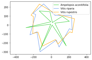
Here, for example, we’re using plt.plot() three times with three different grape species: this is Ampelopsis aconitifolia, Vitis riparia, and Vitis rupestris. We’re giving them each a different color but we’re also using an argument called label. We’re giving this particular data a name and this name is only for this data. You can see the label is just the species name: “Ampelopsis aconitifolia” for the aconitifolia data, “Vitis riparia” for the riparia data, and “Vitis rupestris” for the rupestris data. We have our axis and set_aspect ratio to make our plot proportional.
Because we have this label when we give a name to each of these data sets what happens is when we call plt.legend() we can create a legend and you can choose where it goes. Right now it’s set at lower left. You could say lower right, for example. It even has a option called “best”, so plt.legend() will decide for itself what it thinks is the best location for a legend.
# Use label to create labels for each data element you wish to display in the legend
# Then, use plt.legend() to create a legend and place it

plt.plot(Aaco_x, Aaco_y, color="limegreen",label="Ampelopsis aconitifolia")
plt.plot(Vrip_x, Vrip_y, color="cornflowerblue", label="Vitis riparia")
plt.plot(Vrup_x, Vrup_y, color="orange", label="Vitis rupestris")

# Note in video plt.axes.set_aspect() is used
# But this creates a warning, so gca() (Get Current Axes) is used instead
plt.gca().set_aspect("equal", "datalim")

plt.axis("on")
plt.legend(loc="best") # or "best"
<matplotlib.legend.Legend at 0x7fb97cbeadf0>